TheoLt Release 10 is GO!

Watch this space for full details of the updates, the improvements and how-to’s !

Existing users should contact us now for update details.

TheoLt, TheoLt Contour and TheoLt Tools now improve the productivity of BricsCAD to V17 and AutoCAD to Release 2017 for anyone using Total Station, Laser Distance Meters or Laser Scan Data for the productions of plans or elevations.

TheoContour R10 is coming

No, we do not post often enough here.
No, we do not update our site enough.
Yes we need to work on this.
However you can be sure when we do post, it is important, it is interesting and it is new!

In this case what is new is TheoContour R10!

Its just a week or two away – we are just finishing off the installer and testing the installer.

What can you expect from the new release? You can expect what all software developers say their new releases contain:

  • More Power!
  • More Functions!
  • Easier to Use!Spline-smoothed-6_trimed

In this case it is true! TheoContour (we think) is one of the updates we are most proud of. The new features include:


  • New licensing System (easier to use, more reliable, better trial options).
  • PLY Import
  • Powerful Surface Smoothing Options
  • Powerful Line Smoothing Options
  • Better Layer Control
  • New Surface Creation Options with user definable colours.
  • Better memory management.

Surf ht shaded

Contact Us now for further details!

VirtuSurv Webinar

Webinar introducing functionality of kubit VirtuSurv, high resolution scan data in a simple to use, virtual surveying environment. Connect to any CAD interface including AutoCAD, AutoCAD LT and IntelliCAD. Connect to any Windows based program (Excel, Word and more). Make use of 3D laser scan data without the need for a high level of technical skill. Perform traditional survey from your office.

Traversing with Historic Scotland


Historic Scotland are investing in survey! As part of their development of a minimum site record we do a training exercise in travserse control. I am asked to trouble-shoot their field kit, update to TheoLtr8.1.6 and take 3 teams through network observation and adjustment. The practice site is Blackness Castle and the weather is cold but, mercifully, dry.

We rattle through setting up, do a 4 stn loop, make a mess of station naming, recover and head off to the paraffin perfumed barrack block to check the results. We work through our data and run the calc, the results are superb! The network is adjusted and applied and we enjoy a good buffet lunch before tackling 3 networks in 3 teams.

The new station name editing feature has improved using user defined station names at capture. The great thing about netadjust in TheoLt is the real-time aspect, poor shots are flagged as measured and preview calculations and diagrams can be run, all on live data. Traversing is all about procedure and adapting to new ways of working can make simple things difficult, it always takes patience to get procedures right and we have to make a few re-starts before we get the sequence to suit the situation.

Taking out the ‘brown’ data is a good starting point for analsing the network.

Taking out the poor shots, running the calc and seeing the result can prompt you to take more obs or, in this case,  shave 10ths of a mil off an adjusted station position: a far cry from the days of Bowditch and the calculator!

Because TheoLt works with live station properties station names have been on a like- it -or- lump- it basis until release 8 when it bemame possible to use a custon station name. This is a surprisingly useful improvment as there occasions when station names are pre-set from existing survey or when station ocupation is in decending order, in the past renaming was only possible as an AutoCAD edit post-survey, now the name can be set at Default Orientation or when the station is set out.

Customisable station naming is one method of working with pre-declared station identities, station names can now be determined at setting out adding a new level flexibility to  control operations.

This relatively simple addition to the functionality of Netadjust in TheoLt 8 has a great impact on workflow. Whether you are occupying existing control, adding stations to an existing network or creating a new network from scratch, Theolt now affords the Surveyor the optimum realtime platform for Control networks.

TheoLt Real-Time Network Adjustment offers a new workflow whereby the network benefits from:

  • Review of each observation- Interactive rejection of observations with real-time results update
  • The ability to ensure each station is complete before moving
  • Computation of Resections with multiple face oberservations.
  • Adjustment of CAD drawings to network- Live diagram in CAD

So before you put your kit back in the box you can be sure your network is delivering what you need!

Contouring 5m ESRI GRID data

Recently a 6km2 block of ESRI ASCII Grid 5m demo data has been offered for testing as benchmark for the performance of TheoContour the ‘no frills’ contouring in AutoCAD tool. I’m not sure of the origin of the data but it looks a lot like Lidar and certainly this set gives a good indication as to how TheoContour could handle a 5m post spaced Lidar swath if needed.

The point data is lovely but its dosen’t read like a map and even as a surfaced model it’s not really too useful for mapping so getting countours out of the points is a good first step to getting a map out of it. TheoContour is a great way of making that first step from data to map (getting from points to lines is something of a 1st step in most surveying processes these days!) but the sheer density of the data means a quite bit of care is needed when contouring such a big swath.

the ESRI grid data loaded as AutoCAD points

TheoContour has some slighltly tricky settings and the regular nature of the Lidar data gave me a good oportunity to get some comparative results with the sampling and sub-sampling controls.

The TheoContour contoring controls at 17/17

AutoCAD adressable memory limit: First of all its worth noting that in processing a surface conataining all 237,765 points is a bit like asking TheoContour to hold up the whole sky! It will hit the adressable memory limit in AutoCAD at some point in the calucation process, more than likely this will be at the contour processing end as this is when there is no escape from asking AutoCAD to do a lot of work in plotting the nodes on the contour lines and joining them up. In most cases TheoContour does pretty well at collating the point data so when getting to grips with a big job like this its the contour outputs that test the memory handling in AutoCAD.

First off TheoContour needs to collate the points, this took about 75s and the command line ‘thermometer’ gives you a clue as to what’s going on: running the collate command gives a command line report on completion:

Select points to include in the contour model.
Select objects: ALL
237765 found
Select objects:
Selecting and checking points.
Building Surface.
Checking Surface
Min point 269639.5000, 737484.5000, 105.0000
Max point 272659.5000, 739444.5000, 609.4700
Processed 237769 points,
Boundary Contains 4 points,
Created 475532 surfaces
Average Surface Size: 9.63
Min Surface Size: 5.69
Max Surface Size: 2040.63

This gives us a clue as how to handle this as contours. So the next step is to contour? not quite; with a big processing order like this there will be a limit to what can be done so the choice of contour interval, the smoothing step and processing strategy becomes VERY important at this point! Ignore the need for a suitable interval at your peril:

Plot and join 25million interpolated nodes eh?

Choosing data density over processing capacity: It helps to think of contour generation as ‘node building’ .  The height range is 504.47m from heighest to lowest point ; if we are to contour at a 1m interval we are aking for  503 contour lines, each one ‘joining up’ a rough maximum of  5  points per metre along its length and then interpolating nodes at the changes of direction of the isoline. So an estimate of the required nodes per contour lne might be based on the longest line (say the length of the perimeter in the worst case)  of 10,000m x 5 =50,000 nodes per polyline x 500 polylines =25 million nodes.   For AutoCAD to plot and join 25 million nodes may be possible but my system is best described as ‘average’ (i.e the mininium I can afford for an AutoCAD 20011 platform) so I think working on the basis of a 1m contour interval for the whole block at once is not viable.

A 5m interval would generate 100 contours, an 80% reduction in the amount of processing over 1m. Working with a 5m interval is going to be slow so to test the sampling settings I use a 10m interval. Straight ploylines (splines are very nice but AutoCAD will be pushed hard to generate the smoothing!) with no duplicate point checking further reduces the proessing overheads. Because of the gridded nature of the point data there is a bais to a ‘gridded’ or ‘stepped’ contour model:

10m interval sampling controls at 10/2

10m interval sampling settings at 10/8

By increasing the sub-sampling rate step by step the ‘stepping’ effect of the contours begins to be reduced. Each increase in the sub-sampling rate increases the processing time so there is a point where the sample rate needs to be reduced once a good sub-sampling result is achieved: the goal is to commit to the minimum amount of processing to get the smoothest line. The sub-sampling has the biggest effect on the stepping but aslo the biggest effect on the processing effort.

At 10/17 the contours have lost the stepping and even as straight polylines look like the terrain they depict.

5m 50m idx interval 10/17

With the sampling settings taking up the smoothing the straight polylines work well. The nature of contours is such that the nesting of curves, the pinching of incised features and the moiree effect of lines on convex and concave slopes lead the eye to read the surface as a tactile object. TheoContour generates the lines as polylines so the editing of the lines is not too difficult. Introducing an appropriate  lineweight for the index contour and some sensible colours by layer gets the model behaving cartographically:

5m interval index at 50m

With patience a 2m interval is possible:

2m interval 10m index 10/17

Of course the contours are true 3d enitites:

As you would expect the polylines sit at their correct Zs

2m interval 10m index 10/17

Download TheoContour for Bricscad here.

Dowload TheoContour  (as part of the TheoLt Suite)  for AutoCAD here.

Pointclouds in AutoCAD 2011

One of the (much hyped) new features of AutoCAD 2011 was the inclusion of handling pointcloud data. In this post we will take a quick look at this functionality and how you can make real use of this.

The first issue is that AutoCAD can only read specific (limited) pointcloud formats; LAS, XYB and the 2 Faro formats FLS and FWS. Many users will find this a limitation and need further formats. Further formats may be imported by adding the free version of PointCloud from kubit. The product page is here and the software may be downloadedhere. PointCloud adds the formats PTZ, RiScan Pro and ASCII (CSV, TXT etc).

The workflow of importing pointcloud data is to first index the supplied file to create a PCG file which is Autodesk’s pointcloud format.

This PCG file may be attached in the same way as any other AutoCAD block or image file.

The method of display of the points depends on the current AutoCAD Visual Style. A 2D non-rendered (2D) style displays all of the points in a single colour: black. Selecting a rendered (shaded / 3D) style displays the points in colour.

AutoCAD manages the number of points displayed on the screen. At first loading the density of the points displayed may appear rather thin. Select the density command. Here I have set the value 70. The display is now far more usable. You will find the pan and orbit are very quick and all points within the cloud may be via the Node object snap.

Many will view the fact that AutoCAD can only display the whole cloud or no cloud as a major limitation, this is another limitation that may be bypassed with kubit’s PointCloud software although this further functionality requires the paid version.

PointCloud allows the definition of sections which may be managed in the section manager. These may be created in the following ways;

  • Slice
  • (Shift slice up/down and change slice thickness)
  • (Multiple slices: Parallel or perpendicular to objects/curves)
  • Clipping Box
  • Clipping Polygon (2D projection, inside or outside remains visible).

A typical use of the slice command is to create a plan.

This of course may then be traced. If the version of PointCloud being used is the Pro version then the Automatic Fitting may be used to fit the plan to the slice. This is completed by drawing a very approximate polyline (with the correct number of corners) and selecting the Fit Polygon command.

Working with elevations is a key use of PointCloud data. This however shows another weakness in the AutoCAD  pointcloud display. The density of the data displayed may not be sufficient for tracing details.

Again, PointCloud may come to the rescue here. Using the section manager individual sections of the data set may be saved in PTC format – the native format of kubit’s PointCloud (which enables the support for PointCloud data in AutoCAD’s prior to 2011). The display of the PTC is far denser allowing the details to be seen clearly.

Edit/Note: Release 7, released in May 2011 introduced “SmartSections” a new way of creating and working with this higher density display. The new SmartSections are faster and simpler to use. End Edit/Note.

A further tool within PointCloud is Plane fitting. This enables a plane to be fitted to a number of points and in the case of elevations, the UCS placed on this plane ensuring the elevation is drawn in the correct position.

At first glance it may seem that are are too many disadvantages to using the Autodesk PCG engine and other tools provide a better solution. However when you consider that the PCG engine allows up to 2 billlion points to be inserted into AutoCAD I would suggest that PCG + PointCloud is the ideal tool to manage the dataset within AutoCAD, creating overall plans and views.  with sectioning the data to PTC sections for detail extraction. Take time to download and evaluate PointCloud, again details here.

TheoContour: Fast Contouring made easy!

You can spend a lot of money on contouring, the software tools for surface interpolation and depiction do not come cheap and even the ‘inbuilt’ AutoDesk options require a hefty investment in a ‘Map 3D’ or ‘Civil’ variant. But there is a very effective and low cost option which I have been using for some time now and it’s proved itself to be a good ‘fast and dirty’ fix for getting contours done: TheoContour.

Like all of the Latimer CAD family of tools this is based on the premise of solving a CAD problem, not a surveying one: there are no data tables to code, no CoGo computations to step over and the outputs are pure CAD entities ready for your next DWG based task. And of course all is in 3D from the start.

Let’s start by looking at the results:

This composite view gives you an idea of what TheContour is capable of: annotated smooth 3D ploylines and shaded surface generation.

So how does it work?

TheoContour is an arx/brx application:

it works with points so getting started is easy: just get your points into AutoCAD! The points can be layered anyway you choose, and obviously, they need to be congruent in terms of height consistency ( in other words they have to be organised such that the Z values are correct!)

Once we are happy all the points are in the current view in WCS the 1st TheoContour command is : theocollate which loads up the points and reports on the surface they describe ready for the next step:

I kid you not, the arx processes this stuff pretty quickly 2,703 points in about 3 s!

Note that the command line report relays the settings we are using on this model. They can be changed easily; I’m not happy with contours at 4 to the metre indexed on the metre so I go to settings and switch the index interval to 5:

I’m now ready to contour:

The command is, you guessed it: theoContour! Plotting the contours takes a little time, this example takes about 45s to generate. Some models can take a while, it’s all dependent on how fine the contours are combined the entity type being generated (lines, polylines or splined polylines).

Not bad for a 1st pass, I would return to the settings and look at smoothing but this gives you a good idea of how simple the process is: and it’s flexible- in effect the datum is the zero value for Z in the current UCS so you can use theocontour to generate contoured surfaces indexed to any plane defined by a UCS! The contours are 2D ploylines in 3D space so they can be edited easily using PEDIT to get them tidy!

So just using 2 commands and tweaking the settings I have got working contours in minutes.

TheoContour also generates profiles and shaded surfaces, the text annotation is pretty neat too but for now I just want to show how simple contouring CAN be if you use TheoContour!

TheoContour for BricsCAD

TheoContour can be downloaded as part of TheoLt core at:…

http://www.theolt.com/web/theo-contour/

TheoLt: Powerful Flexible Features.

One of the great advantages of TheoLt compared to other survey software is it’s complete flexibility.  For example, lets take a look at the “Features Library”.

The basic premise of TheoLt is that it transfers the measurement information or point from a survey instrument (or Distance Meter) to CAD to be used by any command  (for example, draw lines, insert blocks etc). What the TheoLt Features Library enables is for a series of measurements to be combined to insert a series of lines, arcs or attributed blocks (much like standard survey “feature coding”).

The feature definitions are accessed through the the settings dialog in the main TheoLt window. Definitions are grouped into folders.

Looking at it’s simplest use, inserting a single attributed block as a detail point. The first stage is to name the feature , define it’s icon and the number of measurements that should be taken to insert the feature. In this case, a single 3D measurement.

The next stage is to define any user attributes that may be required and whether confirmation is required (asking the user to confirm the values). Finally select the block to be inserted.

Once defined, opening the features panel will show the newly created item and a single click on the apropraite icon in the feature  palette will prompt for the measurement and the block will be inserted.

Next we can look at a more complex but typical use; kerbs tops and bottom in topographic survey. The aim here is to pick points on the top and the bottom of the kerbs, connecting the points, inserting blocks and annotating levels. This is very typical of topographic survey. Our definition will be point on top of kerb, point on bottom of kerb before moving on to the next part of the kerb.

Defining the feature, we name it and use 2 3D measurements with correct prompts. As we wish to join the points with lines, we will select “repeat insert” and join points on Layer (each point type having it’s own layer). This will allow the lines to be continued for as many measurements as required before exiting the command.  The attributes will be the Z-level of the first point only and two blocks will be inserted, each on it’s own layer.

Now when selecting the feature from the palate, the measurements are prompted, blocks are inserted and then the first prompt starts again. After the next round of observations, lines are drawn between the respective points on their designated layers. Options allow the lines to be curved, straight  and the alignment of the annotation to be altered or disabled.

The final example is a single complex item; a tree. To measure one fully quite a few measurements are required; the centre of the main trunk, the girth of the trunk, horizontal extent of the canopy and finally the vertical extent (height). These can be defined in the first window with prompts and measurement types. I would assume that for the first measurement the operator would take the angle to the centre of the trunk before taking the distance to the centre. This would leave the instrument pointing to the extent of the girth which we can collect as an angle only measurement. We can also choose to write the details out to a file which can contain any of the collected data fields for processing.

Next we will create the attributes where we will also collect the tree type which will be stored in a list to speed up the user input.

Finally we insert a block to represent the trunk – scaled to match the girth. A second block will be inserted, scaled to math the canopy.  An attributed block is inserted to hold the details of the tree (in addition to the file written above).

Obviously, this is not an in-depth analysis of what is possible from the features palate but I hope it gives some indication of the power within TheoLt.

TheoLt PRO: Traversing

These days big traverses are becoming a rarity. The GPS active net is doing a better job for many survey projects. Traversing is still the best way for getting good control for small sites, setting out, architectural photogrammetry and building survey. I remember the happy time at field school in Wales with booking sheet and pencil, baking in the summer sun, each station in turn becoming a kind of holiday home as we carefully logged back-sight and foresight obs. We got to live outdoors and enjoy it. So, given that this is the backbone of my work, why do I hate it so much?

It is the inevitable disappointment when, at computation, I discover the blunders! All the wonderful effort of getting stations set out, carrying forward heights, multiple obs is lost when the numbers don’t come out! Each time I set out to traverse I have the optimism of a child on a trip to the seaside only to face the bitter disappointment of having to repeat the work to get it right. This is something I have grown used to: traversing is a game of errors and I have, over the years, found out how to get the results I want. In truth I have never been happy with simply surveying for numbers, for me I want to see a drawing, detail, I want that map to grow, to make my mental map real; a schedule of co-ordinates to me is no thing of beauty. So what to do about it?

I can’t do my job without control; I’ll never forget the wise words of Peter Waldhausl when I asked him the teacher’s question: ‘what is the single most important thing to teach in survey?’  his answer, without hesitation, was very clear: ‘NO ACTION WITHOUT CONTROL!’

It’s thrilling to drive in the first peg on un-surveyed territory, this is without doubt part of the elemental appeal of surveying (it’s certainly is NOT the money…few of us are well paid and even fewer of us manage to keep our jobs!) we are part of making the unknown known in a very real way. Anxieties about control can be helped by getting the right tools and first and foremost in these tools is software! I use real-time software that tells me where I’m going wrong when I make the mistakes. Now I know this is not proof against blunder but it definitely helps! Keeping track of where the errors are is one thing but I’m amazed at how much gets in the way of your best rehearsed procedures when you are traversing: for crying out loud there are only 4 things to do:

1. Log the instrument and target heights of collimation (HoC).

2. Achieve and verify orientation.

3. Observe and book shots to back-sight & fore-sight.

4. Set out new station as required.

So what goes wrong?

Plenty! You forget which station you are at and use the wrong station ID, you set out a station then find the sight-line blocked, somebody ( it’s never you!) kicks a tripod and you have to re-set the HoC and retake the station orientation, you select the wrong HoC for the orientation shots, you forget to take the last angle in the loop because you think you already have the shot done as you have ‘been here before’ not to mention the lost marks, last minute datum changes, miss-matched tribrachs, ‘helpful’ people moving setups before they are measured, it starts raining etc.

The software definitely helps, I have a strong tendency to argue with it but I’m learning to trust it (yes I’m pretty stubborn like that I’m afraid).  The Netadjust tool in TheoLt Pro is what keeps my traverses on the straight and narrow.

It has some really good ‘idiot proof’ features which this idiot has learnt to adopt as procedural reinforcement:

Real-time feedback of station selection at occupation and orientation. I get a ‘heads up’ message on completing an orientation that advises me of the staion IDs, the HoCs and the precision of the orientation.

Automatic prompting of HoCs. Every time I take shot to a target I get a prompt, I can turn this off, but this is my most common foul up, its very difficult to ‘unpick’ HoC errors even though it is usually very easy to see where they occur.

Traffic light coloured observation results. This really is the best bit for me, TheoLt will let you know how good your shots are as you take them, you can drop the ‘bad’ obs from the computation, re-shoot or go right back and re-do the orientation again.

Automatic target ID. When you shoot a target with a known position you are prompted with its ID, a simple hint saving a mountain of time searching through tables to find a station ID.

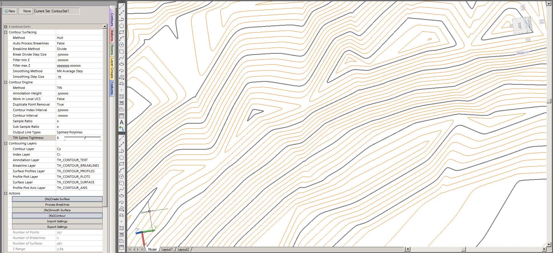
Live diagram. I can preview my loop in AutoCAD/BricsCAD at any time; if it don’t look right it ain’t right. The diagram tells the story.

Non destructive back-up of raw data.  You can run the calc and see what happens at any point in the loop and still have the original observation data logged for QA.

Least squares distribution of error. TheoLt through its partnership with kubit uses a powerful network adjustment algorithm. By moving away from Bowditch (sob!) towards a distributed error network the traverse can be extended to include resections.

TheoLt orientation procedure builds the network data table which shows how good the shots are, how many shots there are in the set and allows you to include or exclude a shot from the computation. I can get reports out on the condition of the network when I run the calc to test the impact of the include/exclude options I use:

Let’s take a look at the report:

TheoLt NetAdjust does traversing nicely but there are drawbacks, its not something I would expect the whole survey world to use. It’s dependent on a PC so its not going to be what I would use on a windswept fellside in driving rain. For me it’s a godsend simply because I can get good control without fuss and move on to what I want to do…draw!

Control networks are essential for a complex building plan. The exterior can often be controlled by a fairly traditional loop with some fun & games to accept GPS points. Once tied to the exterior loop the interior can usually be fixed by resection throughout.

There is always something that gets in the way!

A control network needs to provide points with a higher order of precision than simple polar observations. Easy to say, a fiddle to do, but a whole lot simpler with TheoLt!

www.theolt.com

More on the TheoLt story here:

http://www.caduser.com/reviews/reviews.asp?a_id=187